A Brief Post About K-Means

May 17, 2018 · 6 min read

A few weeks ago I read chapter 4 of the book "Introduction to Applied Linear Algebra" ^[1], called "Clustering," and I found it so clear and simple. Chapter 4 introduces the clustering concept only based on vectors and distance (subjects treated in chapters 1 and 3, respectively) through the canonical example of clustering models: k-means.

In this post I want to make a little review of the chapter and implement k-means in python.

Clustering

The idea of clustering is to partition a set of vectors into $K$ groups based on a distance measurement. An intuitive way to think about it is a 2D-table where each observation (row) is a vector, and we want to assign it to a cluster based on some similarity measurement. So the goal is to add a new categorical variable (column) to the table with $K$ possible group values.

To draw the concept and use an example of the chapter, imagine we are in a hospital and we have a table with measurements of a feature vector for each patient. A clustering method could help separate patients into similar groups and get insights based on these groups. Maybe we could then assign labels and give different diagnosis procedures, and therefore be more effective instead of giving a unique entrance diagnosis.

To formalize what I describe above:

$k$ : a parameter specifying the number of groups that we want to assign.
$c$ : the categorical variable with the group assignation, i.e. a vector with the size of the number of observations.
$G_{i}, i \in (1, \dots, k)$ : a set of indices that represent vectors assigned to group $i$ .
$z_{i}, i \in (1, \dots, k)$ : a n-vector corresponding to group $i$ , this vector has the same length as the vectors we want to assign a cluster.

The similarity within a group $i$ is given by the distance between vectors of a group $i$ and the group representative vector $z_{i}$ . All members share the fact that the distance to this group representative ( $z_{i}$ ) is the minimal one with respect to other group representatives' vectors.

A simple measurement of distance is the euclidean norm defined as:

d (x, y) = | | x - y | | = \sqrt{\sum_{i = 1}^{n} (x_{i} - y_{i})^{2}}

def euclidean_norm(x, y):
    """
    x: a float numpy 1-d array
    y: a float numpy 1-d array
    ---
    Return the euclidean norm between x and y
    """
    return np.sqrt(np.sum((x - y) ** 2))

The clustering objective function ( $J^{c l u s t}$ ) measures the quality of choice in cluster assignments. A better cluster assignment of $x_{i}$ is one where the squared euclidean norm is lower.

J^{c l u s t} = (| | x_{1} - z_{c_{1}} | |^{2} + \dots + | | x_{N} - z_{c_{N}} | |^{2}) / N

Given the nature of the problem, finding an optimal solution for $J^{c l u s t}$ is really hard because it depends on both the group assignation ( $c$ ) and the choice of group representatives ( $z$ ). Instead, we can find a feasible solution for minimising $J^{c l u s t}$ , a suboptimal one (local optimum), by solving a sequence of simpler optimization problems in an iterative approach.

k-means algorithm

Now the way the chapter shows how to assign these $k$ groups is through the k-means algorithm. The best description for k-means is encapsulated in three steps:

Initialize with a fixed set of representatives $z_{i}$ for $i = 1 \dots k$ (pick random observations of the data as representatives, for example).
Now we reduce the problem to just cluster assignations, and we can also see this problem as $N$ subproblems (one for each observation). Just look at which group representative has the minimal distance to vector $x_{i}$ , and assign it to vector $c_{i} : = z^{*}$ .
$| | x_{i} - z_{c_{i}} | | = min_{j = 1, \dots, k} | | x_{i} - z_{j} | |$
The step before gives us a vector with the group assignation ( $c$ ) of each observation ( $x_{i}$ ). Remember that $c$ is a vector of length equal to the number of observations we have in the data. Now, based on $c$ , we come back to the problem of finding a set of group representatives $z$ . This step gives k-means its name, because now we update the set of group representatives by computing the mean of the assigned cluster vectors from step 2.
$z_{j} = (\frac{1}{| G_{j} |}) \underset{i \in G_{j}}{\sum x_{i}}$

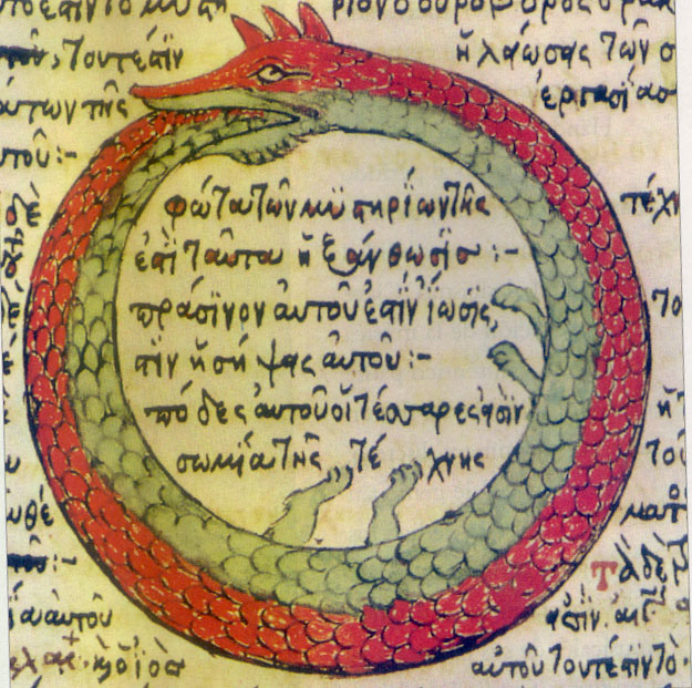
I put the image of Ouroboros above as a graphical analogy, because k-means is self-contained and also iterative — steps 2 and 3 repeat themselves. In each iteration a new assignation of clusters is given, followed by a redefinition of group representatives. But, opposite to the symbolic meaning of Ouroboros, the flow of time is not endless: the process of repetition ends when the algorithm converges to a solution.

When does k-means reach a solution? Convergence occurs when there isn't a variation in the group assignation from the previous iteration ( $c_{t}$ is exactly the same as $c_{t - 1}$ ).

The implementation of the three previous steps is very straightforward using numpy in python:

import numpy as np

def k_means(df, K, num_iter):
    """
    df: a 2D numpy array
    K: number of group representatives
    num_iter: number of iterations to repeat steps 2 and 3
    ---
    Return the cluster assignment (c), group representatives (z), and the
    cost function of each iteration (J)
    """
    nrow = df.shape[0]
    # initialize cluster representatives (STEP 1)
    z = df[np.random.choice(nrow, K), ]
    c = np.empty(nrow, dtype='int64')
    J = []
    iter_counter = 0
    while True:
        J_i = 0
        # solve the N subproblems of cluster assignation (STEP 2)
        for j in range(nrow):
            distance = np.array([euclidean_norm(df[j, ], z_i) for z_i in z])
            c[j] = np.argmin(distance)
            J_i += np.min(distance) ** 2
        J.append(J_i / nrow)       # cost function evolution by iteration
        # update group representatives, take the mean based on c (STEP 3)
        check_z = np.array([np.mean(df[c == k, ], axis=0) for k in range(K)])
        if np.all(np.equal(check_z, z)):       # check convergence status
            # reached convergence
            break
        if num_iter == iter_counter:
            # stop the process at iteration number -> iter_counter
            break
        z = check_z
        iter_counter += 1
    return c, z, J

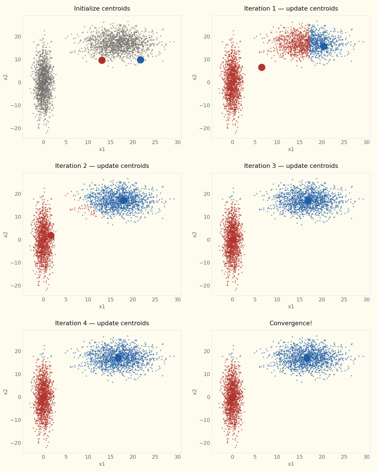
A good way to understand k-means is visually and step by step! So I wrote k_means with the argument num_iter, which allows stopping the process at a certain iteration and getting the results at that point.

We can play with the algorithm and show the evolution of centroid definition and cluster assignation, but before that we need some data. We generate two groups of random data $D \in R^{2}$ from two bivariate normal distributions with the following parameters:

\begin{matrix} µ_{0} = (0, 0) µ_{1} = (17, 17) \\ σ_{0} = [\begin{matrix} 1 & 0 \\ 0 & 50 \end{matrix}] σ_{1} = [\begin{matrix} 15 & 0 \\ 0 & 12 \end{matrix}] \end{matrix}

A simple dataset with 2 features helps us to visualize it easily. Additionally, we know a priori that there are two underlying groups, since these are defined by the two different distributions. If we look at the next plot, both samples are well separated into different groups. This is a very basic setting, but the purpose is to illustrate how k_means works.

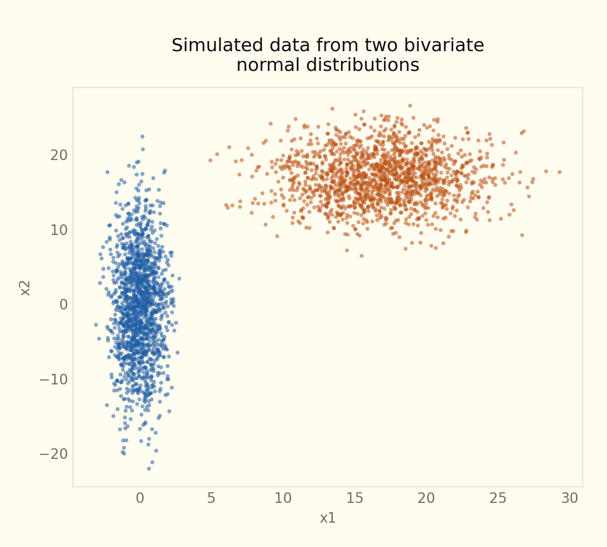
So k_means is blind to the colours, and its goal is to uncover the samples generated by the two underlying distributions based only on the data. Pictorially, the process looks like this:

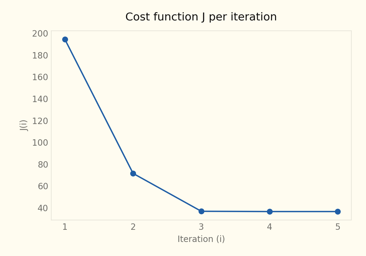
For the cost side, $J$ decays rapidly and converges around a cost value of 36:

J
> [194.43, 71.56, 36.85, 36.61, 36.61]

Additional resources

kmeans.py — the script used to regenerate the plots and the animation above in pure Python. The original 2018 version of this post was an .Rmd (R + reticulate) that ran this same k_means implementation but rendered every plot through ggplot2, stitching the per-iteration PNGs into a GIF with an external tool.

References

Boyd, S. & Vandenberghe, L. (2018). Introduction to Applied Linear Algebra: Vectors, Matrices, and Least Squares. Cambridge University Press.