A Deep Learning Workflow Part 1, Hugging Face datasets + Weights & Biases

Example Project: Fine-Tuning an Image Segmentation Model

Our project today involves fine-tuning an image segmentation model (SegFormer) with cellular images from a high-throughput microscope 🔬.

The idea is to train a model using cellular photography with mask labels that denote the living cells. A good model can connect directly to the microscope and help scientists detect cells quickly affected by a given treatment.

We are talking about reproducibility and collaboration so that you can follow the Google Collab Notebook (it’s the same at the banner at the start of the post). The notebook has three sections:

1. Image Segmentation Walkthrough with SegFormer 📸: Model usage on this specific domain task and how the dataset interacts with them.
2. Training + Weights & Biases experiment tracking 🪄 + 🐝: training, hyperparameter optimization, and experiment tracking using Weights & Biases (W&B).
3. Training script via command line 🚀: A section to experiment with different model configurations using a training script.

These three sections broadly follow the development of the project. First, we’ll understand how to use the model and the dataset manipulation to feed it. Next, we’ll start working on training, namely what we want to track and record, and the hyperparameters configurations (such as the learning rate and batch size).

These two initial sections work as an internal exploration and as documentation for anyone who wants to understand the project. The third and final step is an engineering effort to make life easier and get the job done.

Hugging Face Datasets

If you’ve dabbled in machine learning, chances are you’ve worked on the classic MNIST dataset alongside PyTorch. The code below makes this easy so you don’t have to run boilerplate code or download MNIST every time you want to experiment. You can instead focus on learning new models and concepts.

import torchvision.datasets as datasets
MNISt=datasets.MNIST(root='./data', train=True, download=True, transform=None)

In the same spirit of pulling MNIST from PyTorch, we want our data for this project in a central repository, ready to consume, and easy to share. We can get these three features for free using the HuggingFace dataset repository.

In Figure 2, we have a picture of the dataset repository of the example project, a page where you have a preview and documentation of the data. There is also a repository for storing images, text, or other data you have and there is no limit size for the data storage reported in the documentation. Still, I created a repository that stored the NIH Chest X-ray dataset (> 40gb) without problems, and there are datasets with terabytes of memory.

The purpose of investing time in creating a repository for your dataset is that you’ll end up with a Python module for downloading and loading the data in the same fashion that torchvision.datasets provides you with the MNIST and others benchmark datasets.

Below you can see how we load the dataset for the cell segmentation example project:

from datasets import load_dataset

repo_name = "alkzar90/cell_benchmark"
train_ds = load_dataset(repo_name, split="train", streaming=False)
val_ds = load_dataset(repo_name, split="validation", streaming=False) 
test_ds = load_dataset(repo_name, split="test", streaming=False) 

How does HuggingFace know how the dataset load (i.e. read files and split the data)?

1. The module supports common data types by default, such as tabular, images, text, audio, etc. You need to follow a template for storing the organized dataset, something like torchvision.datasets.ImageFolder approach (i.e. data_split/label/image_001.jpg). This helps the Hugging Face dataset module figures out how to load your data.
2. Sometimes you must accommodate multiple datatypes (CUB 200 2011 dataset), or you might want to provide different configuration of the dataset for various tasks such as image classification and object detection (in the dataset preview rock glacier dataset, notice the data subset option), or your dataset type lacks default support by the library. In this case, you must write a custom python (simple example / complex example) loader script to tell the module how to navigate the file structure, deal with data and labels.

The datasets repository works similarly to a GitHub repo. You can get version code and data with commits, collaborate with others via pull requests, and have README for general dataset documentation. There is also support for apache arrow format to get the data in streaming mode, Finally, when the data is too heavy to load at once, you can download it, and via the caching system, you can load batches on demand in memory.

Experiment tracking with W&B

Weight & Biases (W&B or wandb) provides free services for logging information about your project into a web server that you can monitor from a dashboard. It’s helpful to think of your W&B project as a database with tools for interacting with your experiment information.

Once you have a W&B account, you can create a project such as alcazar90/cell-segmentation to log the information from each experiment you run.

In section 2 of the google colab, sub-section “🦾 Run experiment”, you’ll initialize a run with wandb.init providing the following arguments: (i.) name of the project and (ii.) a config dictionary that provides context about your experimentation such as number of epochs, batch size, etc. Also, you can name your runs something memorable, but if you don’t, W&B create random expressions such as resplendent-rocket-27 or abundant-moon-38 (yes, the number is the experiment number).

Commonly, there will be a lot of runs in your project because when you get a taste of the improvements in you can make in how you log information, you’ll find yourself getting a ton of new ideas.

PROJECT = 'cell-segmentation'
wandb.init(project=PROJECT, config={"epochs": EPOCHS, "batch_size": BS, "lr": LR,
                                    "lr_scheduler_exponential__gamma": GAMMA, 
                                    "seed": SEED})

# Add additional configs to wandb if needed
wandb.config['len_train'] = len(datasets.train_ds)
wandb.config['len_val'] = len(datasets.valid_ds)

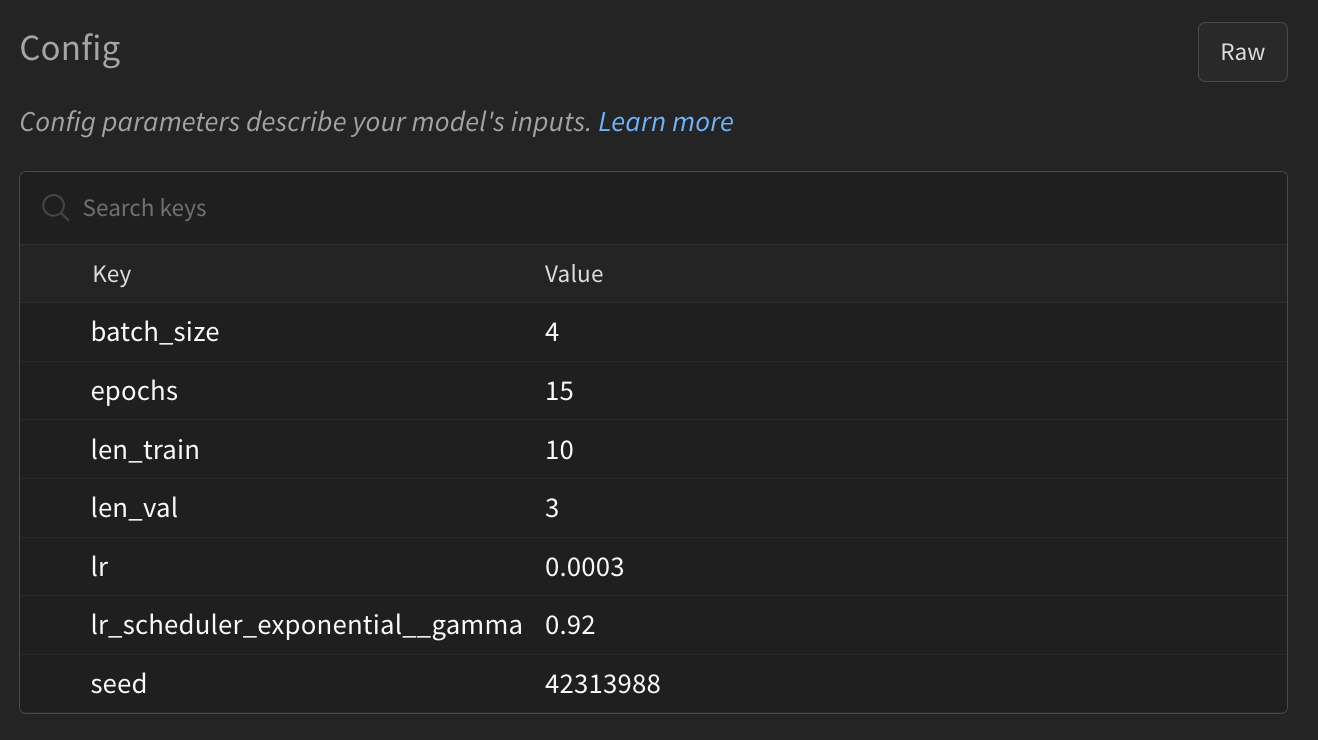
For example, you can see the config information in the dashboard from the run auspicious-paper-44 in the overview option at the left menu. There is a table describing the context of this experiment (mostly hyperparameters settings in this case):

After initializing a run and logging the config, we want to log information during the model training. Typically we want to track the main metrics in the train and validation set; these will be floating points across time that we log using wandb.log.

for epoch in tqdm(range(EPOCHS)):
  ...
  metrics = {"train/train_loss": train_loss, 
               "train/epoch": (step + 1 + (n_steps_per_epoch * epoch)) / n_steps_per_epoch, 
               "train/example_ct": example_ct,
               "train/cur_learning_rate": scheduler.state_dict()["_last_lr"][0]}
  ...
  val_metrics = {"val/val_loss": val_loss, 
                 "val/val_accuracy": accuracy,
                 "val/mIoU": mIoU}
  wandb.log({**metrics, **val_metrics})

W&B knows how to display these metrics, so it makes charts for you automatically in the run’s dashboard.

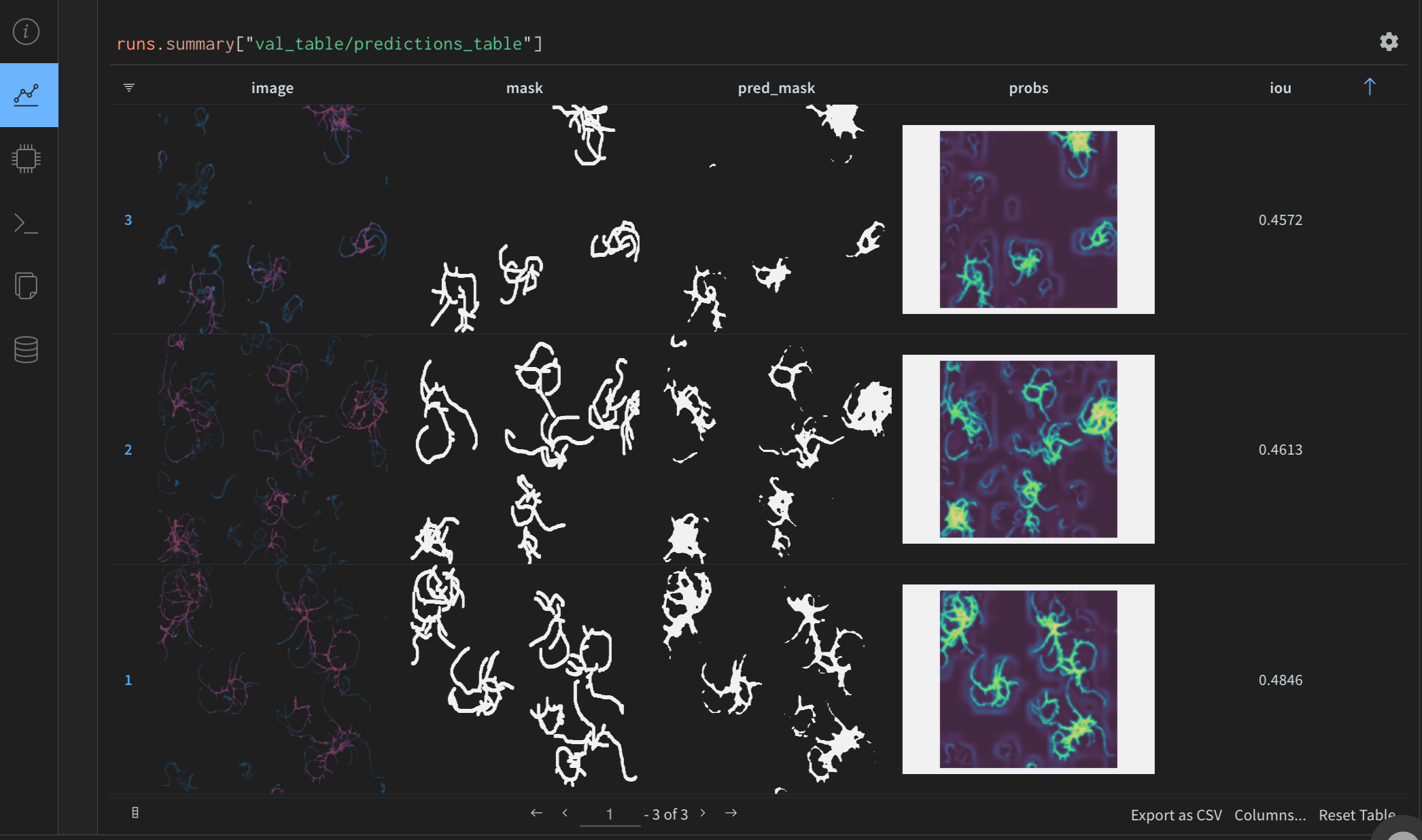
Beyond the obvious things to log (like training and validation loss), you can log whatever you want for your specific project. In the Figure 5, I log information from the dev set into a wand.Table includes:

• The actual image and mask
• The predicted mask
• The probability map (it’s so cool)
• The intersection over union (iou) metric for individual examples

# 🐝 Create a wandb Table to log images, labels and predictions to
table = wandb.Table(columns=["image", "mask", "pred_mask", "probs", "iou"])
for img, mask, pred, prob, iou_metric in zip(images.to("cpu"), masks.to("cpu"), predicted.to("cpu"), probs.to("cpu"), iou_by_example.to("cpu")):
    plt.imshow(prob.detach().cpu());
    plt.axis("off");
    plt.tight_layout();
    table.add_data(
      wandb.Image(img.permute(1,2,0).numpy()), 
      wandb.Image(mask.view(img.shape[1:]).unsqueeze(2).numpy()),
      wandb.Image(np.uint8(pred.unsqueeze(2).numpy())*255),
      wandb.Image(plt),
      iou_metric)

Notice in the code that wand.Table has image columns that we add using wand.Image and requires numpy arrays as input, but you can also log plots created with matplotlib, like in the case of the probability column. These allow us to have tables with rendered images as values that we can inspect quickly. This feature is convenient as a complement to traditional metrics. However, for generative image models, checking the pictures you generated by the model during training gives you more information about your model than tracking the loss.

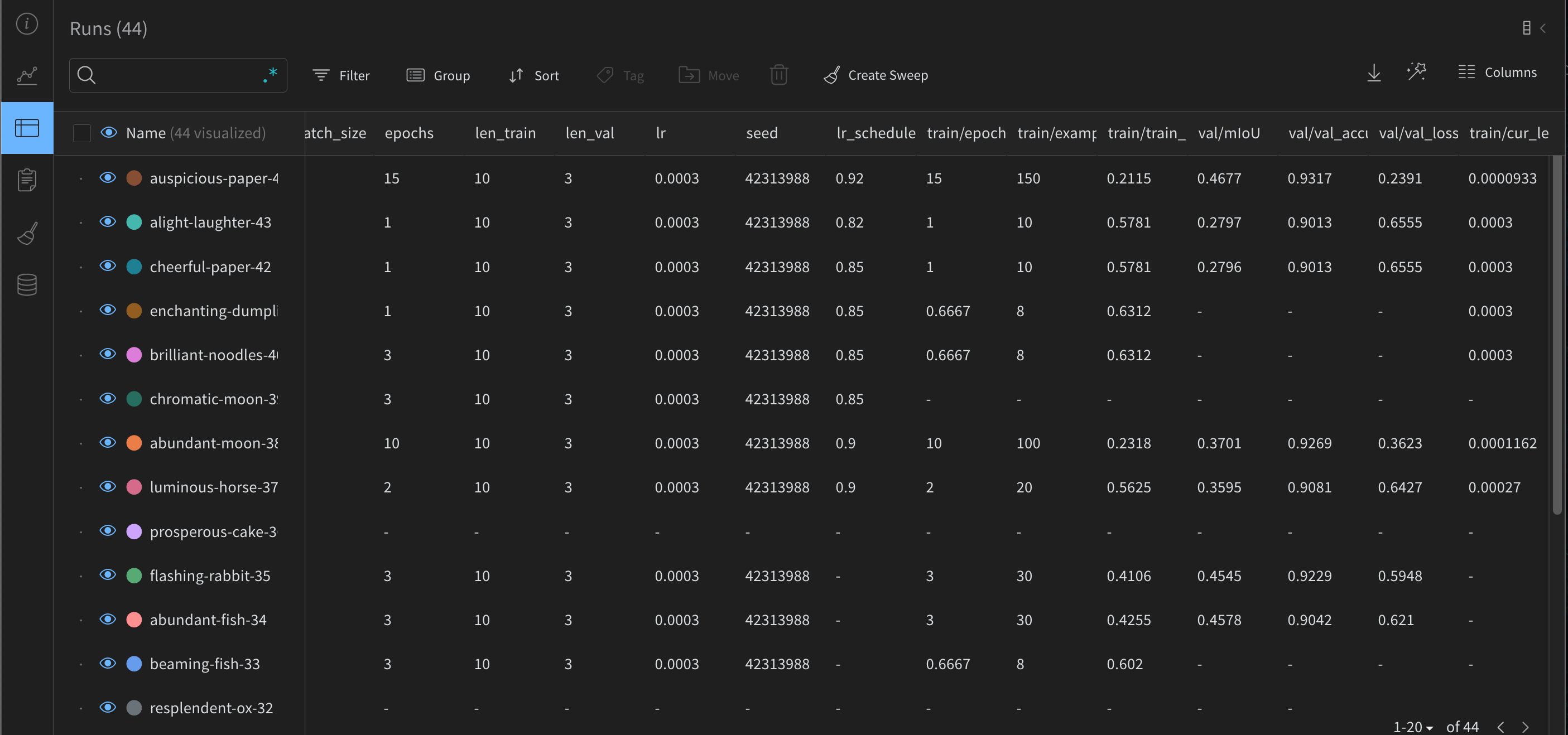
Finally, on your project’s main page, in the “Table” option at the left menu, you have a bird-eye view of all runs and their metrics to compare. You can export this info into a csv file or download it by API to analyze.

Note 1: Whenever you initialize a run (wandb.init), W&B will ask you to provide the API key for authentication; you can find it at W&B>settings>API keys.

Note 2: There is a short course of W&B called “Effective MLOps: Model Development” to learn the fundamentals.

Training Script Via Command Line 🚀

In the last section, we saw how to integrate W&B to log information about our model training. Still, fine-tuning a model or training from scratch requires a lot of experimentation. The idea is to iterate and try many configurations.

And sure, you can do this in the notebook, but doing it that way is redundant and non-optimal. Think about re-running every time the code cells after you change the batch size in your data loaders, for example. That’s not ideal. The next step is to wrap all the code cells required to train your model into a training script, such as downloading the dataset, creating the data loaders, importing utility functions, and setting hyperparameters and training configurations.

Wrapping the code into a training script, plus using the argparse module, you’ll be able to call the training script directly from the command line:

!python finetune_model.py --train_batch_size 4 --validation_batch_size 3\
     --init_learning_rate 3e-4 --learning_rate_scheduler_gamma 0.92\
     --num_train_epochs 15 --reproducibility_seed 42313988\
     --log_images_in_validation True --dataloader_num_workers 0\
     --model_name "huggingface-segformer-nvidia-mit-b0"\
     --project_name "cell-segmentation"

You can see the training script here, but the main heavy work is done by the argparse module where you can define a parser protocol to define and read the parameters for running the script via the command line. The idea is as follows:

import argparse 

def parse_args(input_args=None):
  parser = argparse.ArgumentParser(description="Training loop script for fine-tune a pretrained SegFormer model.")
  
  parser.add_argument(
    "--train_batch_size", type=int, default=4, help="Batch size (per device) for
    the training dataloader"
  )
  ...

Thus far, we’ll developed the entire code project in Google Colab, created a HuggingFace dataset repository, and integrated W&B to log the model training information. But the project doesn’t have any home in GitHub.

When is it actually necessary to create a code repository for the project? It depends. For example, if creating the dataset requires pre-processing scripts and tests, keeping all those files in a GitHub repository makes sense. Regardless, the moment we develop the training script, creating a GitHub repository for the training script and its dependencies is a good decision. We want to make the training script accessible, even for us. In the last section of the google colab notebook, I downloaded the training script from the GitHub repo to train using the computation provided by colab.

!wget https://raw.githubusercontent.com/alcazar90/cell-segmentation/main/finetune_model.py

Side actions to do with your repo: upload a Jupyter notebook version of the Colab and write a nice readme to provide context.

Next Steps 🦶🏼

If you (or I) wanted to continue the project, some next steps to consider:

1. Create a bash script for running a .txt file with different training configurations.
2. Create files to separate code from training.py, such as model.py for code related to downloading and loading models and inference.py for computing evaluation metrics.
3. Use a cloud provider such as Lambda Cloud to connect via ssh and run the training script. Check if the results save in W&B.
4. Explore how to use Hugging Face GitHub actions/webhooks to save model checkpoints in HF every time the training script outperforms the current best model. Check hugging face sync action, and HuggingFace Webhooks
5. Study cases for popular deep learning code repositories such as the OpenAI whisper model and nanoGPT.

Conclusion

Using W&B and Hugging Face makes projects like the one above a lot easier to manage, reproduce, and understand. Having the code ready in a Colab gives us GPU access and makes running discrete steps a breeze.

I hope this piece helps you as you consider how best to experiment in your project. If you have any questions, feel free to drop them in the comments below. Thanks!